This webpage provides supplementary information and data for the paper:
Elastica: A compliant mechanics environment for soft robotic control.Code to run the four cases presented in the paper is available on Github here while results data for the tuning of hyperparameters and other parameters (such as control points in Case 3) along with Jupyter notebooks for their analysis are available here.
On this page we provide some additional details on how exactly we set up the different cases, unpack and discuss some of the hyperparameter tuning results, and provide some extra implementation details in order to help others reproduce (and expand upon) our results.
- Case 1: 3D tracking of a randomly moving target
- Case 2: Reaching to random target location with defined orientation
- Case 3: Underactutated maneuvering among structured obstacles
- Case 4: Underactutated maneuvering among unstructured obstacles
- RL methods for control of soft, compliant robots
- Elastica implementation details
Case 1: 3D tracking of a randomly moving target
Problem Description:
The goal of this case is for the tip of the compliant arm to continuously track a randomly moving target in 3D space. The target moves with a constant velocity of 0.5 m/s while randomly changing directions every 0.7 seconds.
Actuation (Action) Definition:
Actuation is allowed in only the normal and binormal plane, with the applied torque in each direction controlled by 6 equidistantly spaced control points leading to a total of 12 degrees of freedom.
State Definition:
The state $S$ of the system is defined by the 44 element array: $S = \left[x_a, v_a, x_t, v_t\right],$ where $x_a$, $x_t$ describe the three-dimensional position of the arm and the target, and $v_a$, $v_t$ describe the magnitude and the direction of the velocity of the tip of the arm and the target. Note that $x_a$ is constructed by taking multiple (in our case, 11) equidistant points along the arm to keep the dimensionality of the state low while maintaining enough information.
Reward Function Definition:
The reward function is designed to reward the agent for minimizing the distance between the tip of the arm and the target. It is defined as
$R = -n^2 + g(S) + \begin{cases} 0.5 & d<n<2d\\2.0 & n<d\end{cases}$
where $n$ is the square of the L2 norm distance between the tip of the arm and the target $n = || x_n - x_t ||$ and $d$ is a defined bonus range distance (here $d$ = 5 cm). Additionally, because the allowed action space was capable of causing the simulation to become unstable, a penalty term of -1000 was added any time a NaN was detected in the state information, which indicated the simulation had become unstable. Detection of a NaN would cause the episode to end.
Hyperparameter Tuning:
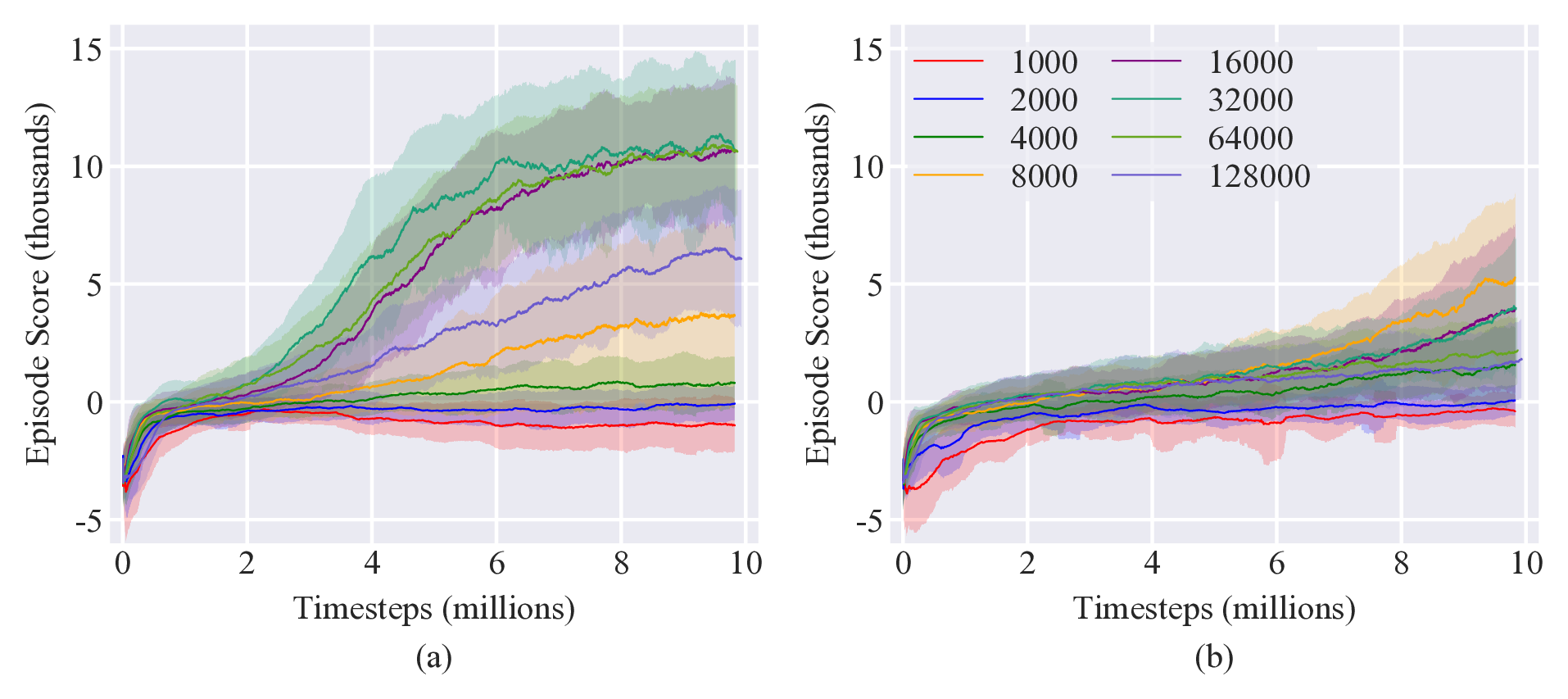
Only a single hyperparameter was tuned for each algorithm. For the on-policy methods (TRPO and PPO), the batch size was varied between 1000 and 128,000 with policies trained for 10 million timesteps and with 5 different random seeds. Results are shown in Figure 2. For PPO, there was a poor performance for small batch sizes, to the point the policy was not able to achieve a positive episode score, indicating that it failed to complete the task. Performance increased with increasing batch size, peaking with similar performance for batch sizes of 16,000, 32,000, and 64,000 before decreasing for a batch size of 128,000. Similar trends were observed for TRPO, though with a batch size of 8000 outperforming all others.
For the off-policy methods, the replay buffer size was varied between 100,000 and 2 million. Policies were trained for 5 million timesteps with 5 different random seeds (it was found that off-policy methods took about twice the compute time as on-policy methods). Results are shown in Figure 3.
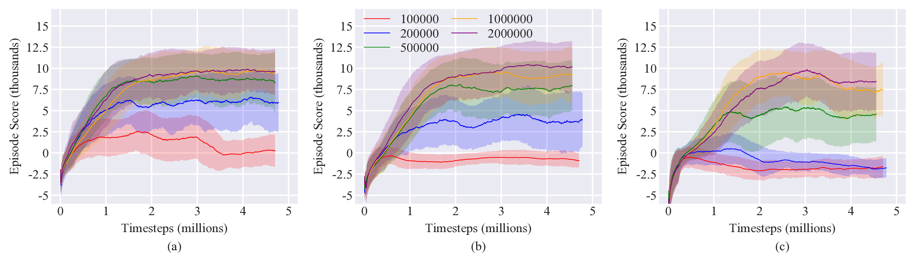
The improvements of the algorithms with increasing batch size and replay buffer size are intuitive when considered in light of the varying random target location. The effect of both larger batch sizes and replay buffers is similar in that target locations from a wider variety of locations are included in the policy optimization (since more time will have passed to allow the target to have moved around).
Case 2: Reaching to random target location with defined orientation
Problem Description:
The goal of this case is to have the tip of the arm reach towards a stationary target location that is randomly positioned every episode. Additionally, the arm needs to orient itself to conform to a target orientation. The target orientation is defined such that the tangent direction of the arm tip should be pointed vertically upwards while the normal-binormal vectors are rotated away from the global coordinate frame (also the initial coordinating frame of the tip) by a random amount between $-90^{\circ}$ and $90^{\circ}$.
Actuation (Action) Definition:
In this case, in order for the arm to match the prescribed orientation, it is necessary to include twist in the possible actuations. Similar to the normal and binormal actuations of Case 1, the twist of the arm is controlled by 6 equidistantly distributed control points. This, combined with the same normal and binormal actuations of Case 1, led to 18 control degrees of freedom.
State Definition:
The state $S$ is the same as in Case 1 (3D tracking of target), where $x_a$, $x_t$ describe the three-dimensional position of the arm and the target, and $v_a$, $v_t$ describe the magnitude and the direction of the velocity of the tip of the arm and the target, but with the addition of two quaternions that describe the orientation of the coordinate frames of both the tip of the arm ($q_a$) and the target ($q_t$) $S = \left[x_a, v_a, q_a, x_t, v_t, q_t\right]$ leading to a state size of 48 elements.
Reward Function Definition:
The reward function is similar to that used in Case 1 but with an additional penalty term proportional to the difference between the orientation of the tip of the arm and the target orientation along with bonus awards as the two orientations approach each other. A continuous and sparse penalty term is added to the reward term to align the orientation of axes of the tip of the arm and the target. The orientation penalty is $p = 1 - (q_a \cdot q_t)^2$, leading to a graded reward
$R = -n^2 - 0.5 p^2 + g(S)+ \begin{cases} 1.0 - 0.5p & d<n<2d \text{ and } p>0.1\\1.5 - 0.5p & d<n<2d \text{ and } p<0.1\\4.0 - 2.0p & n<d \text{ and } p>0.1\\4.5 - 2.0p & n<d \text{ and } 0.05<p<0.1\\6.0 - 2.0p & n<d \text{ and } p<0.05 \end{cases}$
where $n$ is the square of the L2 norm distance between the tip of the arm and the target $n = || x_n - x_t ||$ and $d$ is a defined bonus range distance (here $d$ = 5 cm).
Hyperparameter Tuning:
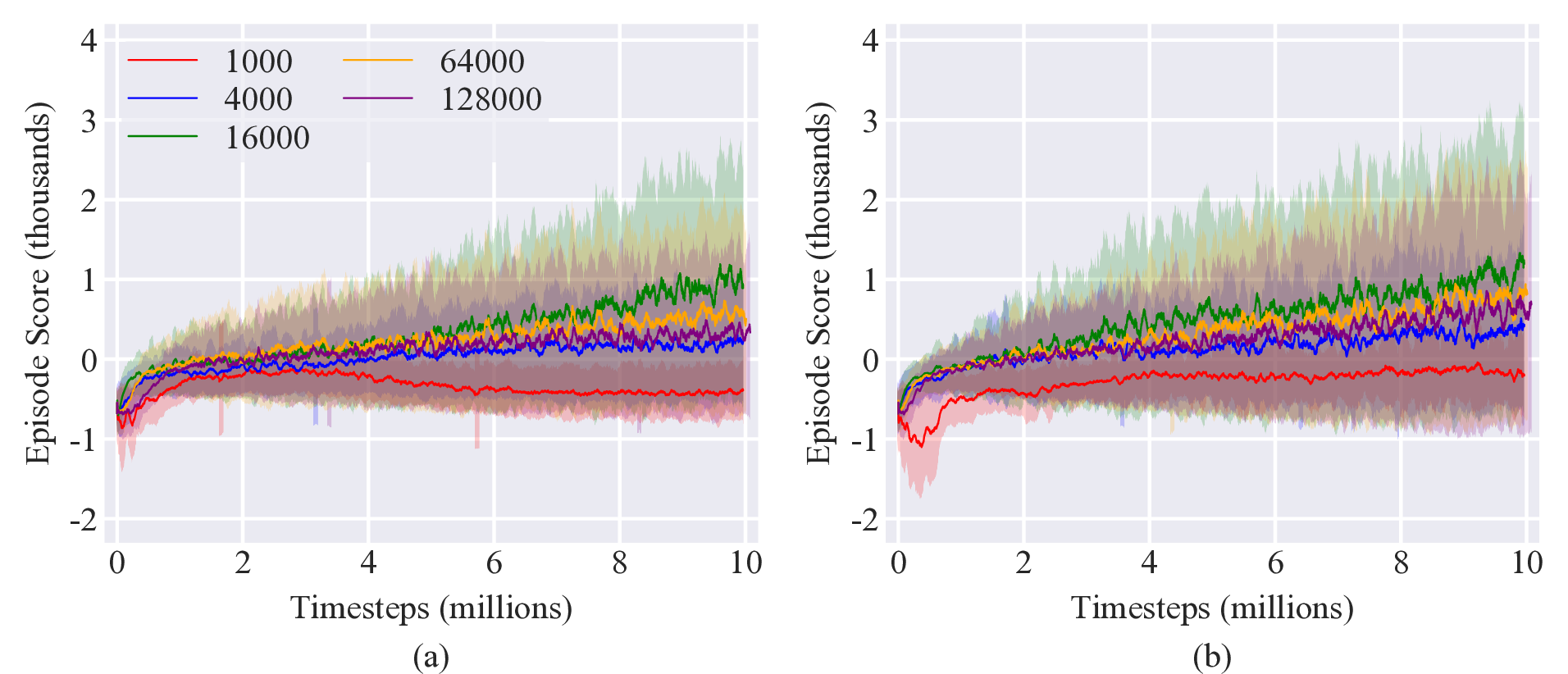
Only a single hyperparameter was tuned for each algorithm. For the on-policy methods (TRPO and PPO), the batch size was varied between 1000 and 128,000 with policies trained for 10 million timesteps and with 5 different random seeds. Results are shown in Figure 4. For PPO, there was a poor performance for small batch sizes, to the point the policy was not able to achieve a positive episode score, indicating that it failed to complete the task. Performance increased with increasing batch size, peaking with the best performance for a batch size of 16,000 before decreasing as the batch size continued to increase. Similar results were observed for TRPO.
For the off-policy methods, the replay buffer was varied between 100,000 and 2 million. Policies were trained for 5 million timesteps with 5 different random seeds (it was found that off-policy methods took about twice the compute time as on-policy methods). Results are shown in Figure 5, exhibiting similar trends as the hyperparameter tuning results of Case 1.
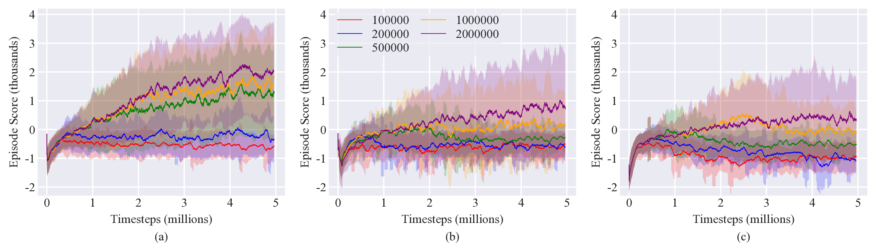
The improvements of the algorithms with increasing batch size and replay buffer size seen here in Case 1 can be explained via the same rationale as with Case 1. Here, the improvement is more pronounced, explained by the fact that the target location is stationary during each episode, necessitating samples from many episodes be included in the policy optimizations for the policy to learn to generalize to a random target location.
Case 3: Underactutated maneuvering among structured obstacles
Problem Description:
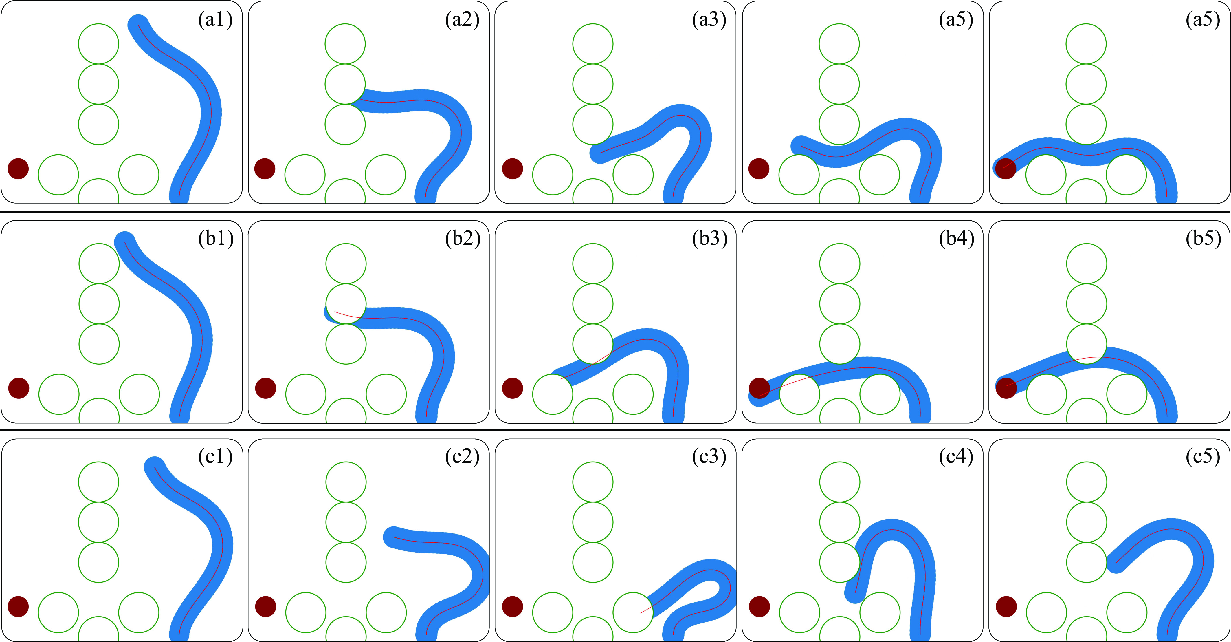
In this case, a stationary target is placed behind an array of 8 obstacles with an opening through which the arm must maneuver to reach the target. The target is placed in the normal plane so that only in-plane actuation is required. Obstacles and target locations are located in the same location and configuration each episode. In this case, obstacles are placed so that there is only one possible way for the arm tip to reach the target. Contact between the arm and obstacles is modeled via a repulsive contact force explained in here.
Actuation (Action) Definition:
Because the target was placed in the normal plane, the problem is essentially a 2D reaching problem. As such, only actuation in the normal direction was enabled. To explore the interplay of underactuation and environmental interaction, 2 control points manually placed at locations 0.4L and 0.9L along the arm were used. Additionally, simulations were performed for different control point setups with policies trained for 2, 4, and 8 equidistantly located control points. Due to their out performance of the off-policy methods in the presence of obstacles, only TRPO and PPO were used to investigate these different number of control points. Results are shown in in Figure 6.
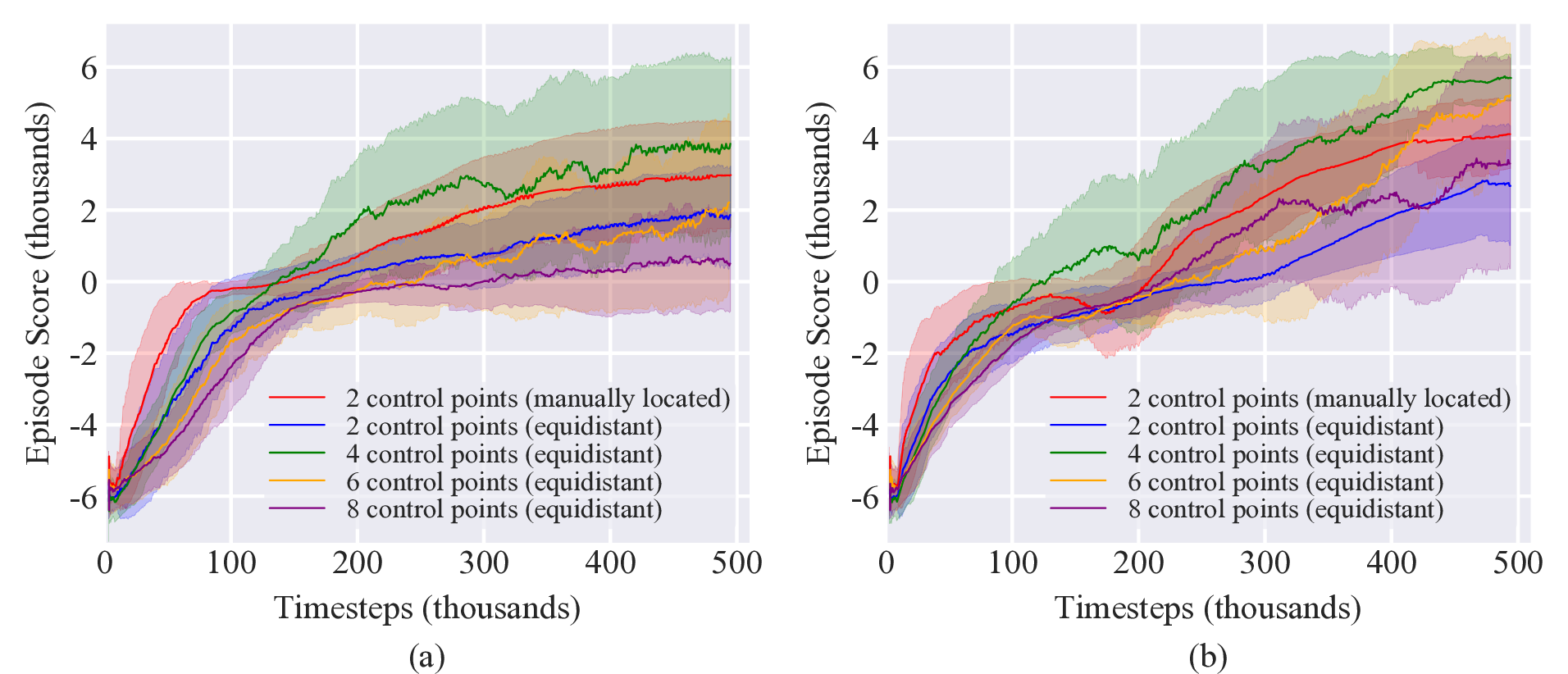
The results in Figure 6 indicate that poor performance was achieved for both 2 and 8 equidistant control points. This result is intuitive as 2 equidistant control points does not provide the proper amount of control for the tip to reach the target while 8 control points has a larger action space that must be explored, leading to slow learning. 6 control points performs better than 8 control points due to its smaller action space while 4 control points achieves the best performance as it strikes a balance between having sufficient actuation to complete the task and a small enough action space to allow fast exploration.
Notably, the two case with manually placed control points also performs well, with a final score between that of 4 and 6 control points. This was possible because the manually placed control points were located so as to exploit the compliance of the arm and maximize its controllability with the fewest possible number of control points. One control point was placed near the middle of the arm (40% of the arm length) to generate large bends and so control gross deformation of the arm. The second control point was placed close to the arm tip (90% of the arm length) to control its sliding direction when pushing along obstacles as well as enable fine tip control in order to reach the target after maneuvering through the obstacles. Fewer control points enables faster action space exploration, resulting in more sample-efficient learning. Note that the 2 manually placed control points outperforms the learning performance of the 4 control points setup over the first 100k timesteps before the increased controllability of the 4 control points ultimately enables it to achieve higher scores.
State Definition:
The state $S$ is similar to that of Case 1 (3D tracking of target) (where $x_a$, $x_t$ describe the three-dimensional position of the arm and the target, respectively and $v_a$, $v_t$ describe the magnitude and direction of the velocity of the tip of the arm and the target, respectively) but with the addition of the location of the obstacles $x_{obs}$. The obstacles are cylinders and the location of the $n$^th^ obstacle is represented by 5 equidistant points along the obstacle $( x_{obs}^{i,n}, \ \ i=0,\dots,4)$. The state is then defined as the array $S= \left[x_a, v_a, x_t, x_{obs}^{i,n}\right] {.}$ Because the target is stationary, the target velocity $v_t$ was not included in the state. Eight obstacles were used in this case leading to a state size of 80.
Reward Function Definition:
The reward function is designed to reward the agent for minimizing the distance between the tip of the arm and the target. It is defined as
$R = -n^2 + g(S) + \begin{cases} 0.5 & d<n<2d \\ 2.0 & n<d \end{cases}$
where $n$ is the square of the L2 norm distance between the tip of the arm and the target $n = || x_n - x_t ||$ and $d$ is a defined bonus range distance (here $d$ = 5 cm). Additionally, because the allowed action space was capable of causing the simulation to become unstable, a penalty term of -100 was added for any time a NaN was detected in the state information, which indicated the simulation had become unstable. Detection of a NaN would cause the episode to end. A lower instability penalty term was used in these simulations than in Case 1 and 2 because in those cases instabilities are generally due to action selection that results in large force variations, which is not useful in solving the given problems and so should be fully avoided. In contrast, here instabilities often arose due to interactions with the obstacles. Interaction with obstacles is essential to solving the problem and so should not be so strongly penalized that the agent avoids obstacles altogether.
Hyperparameter Tuning:
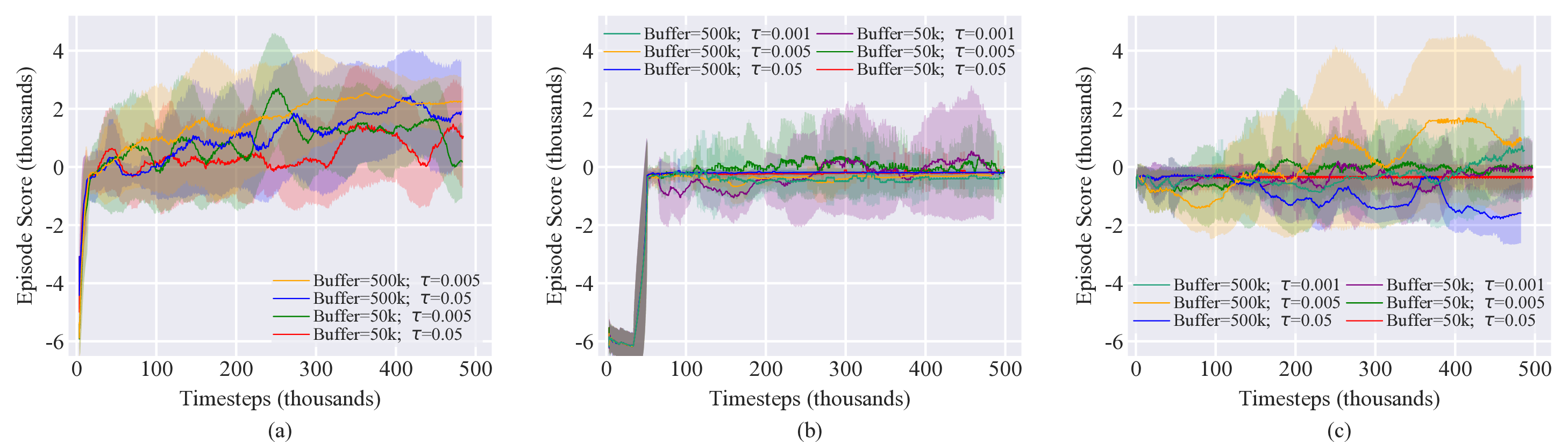
Limited hyperparameter tuning was performed for this case. The on-policy methods used the hyperparameters identified in Case 2 with a batch size of 16,000. For the off-policy methods, the replay buffer as well as the soft update coefficient $\tau$ were varied between two values. Results are shown in Figure 7. Hyperparameter tuning was generally inconclusive with limited improvement seen. DDPG and SAC do appear to perform better with a larger batch size, while TD3 does not exhibit much improvement for different batch sizes. Generally, the best performance was achieved for $\tau=0.005$ for SAC and DDPG and $\tau=0.001$, though there is not a strong dependence.
Modeling obstacles with penalty term instead of contact force:
As discussed in the paper, a key reason the compliant arm is able to solve Case 3 is because its interaction with its environment is included in the model, enabling it to exploit its compliance to interact with the obstacles and allowing it to solve the task with only 2 DOFs. Traditional methods of dealing with obstacles attempt to avoid them by imposing penalty terms. This approach is sufficient for rigid-link robots because interactions with obstacles are undesired due to their ability to damage either the robot or the obstacle. However, such an approach does not allow a compliant robot to fully exploit its compliant properties. To demonstrate this, we retrained a PPO algorithm (with the same hyperparameters as in the paper) to attempt Case 3, however, without modeling the interaction of the arm with its environment but rather incorporating a penalty term into the reward function to account for intersection with obstacles. The new reward function is
$R = -n^2 -\phi f(S) + g(S) + \begin{cases} 0.5, & d<n<2d.\\ 2.0, & n<d. \end{cases}$
where $\phi$ is an intersection penalty coefficient and $f(S)$ is an intersection checking function. Two different $\phi$ values were used ($\phi=10$ and $\phi=100$) to examine the behavior for a lightly-penalized and a heavily-penalized system. Figure 8 compares the result of an arm that is able to interact with its environment and the two cases that account for obstacles via reward penalties. In the case of the lightly-penalized system, the arm learns that the penalty from the obstacles is less than the reward for reaching the target and so intersects the obstacles to reach the target. In the heavily-penalized system the penalty is so large that the arm becomes unwilling to approach the obstacles. In neither case is the arm able to avoid intersecting the obstacles and also reach the target. This is unsurprising due to it only having 2 DOFs and so not enough controllability to perform the precise maneuvers necessary to complete the task. These results underscore how it is only through considering interaction with the environment that the unique capabilities of compliant robots can be realized.
Case 4: Underactutated maneuvering among unstructured obstacles
Problem Description:
The goal of this case is to have the tip of the arm reach towards a stationary target by maneuvering around an unstructured nest of 12 randomly located obstacles. Obstacles and target locations are located in the same place and configuration each episode. Contact between the arm and obstacles is modeled via a repulsive force explained in here.
Actuation (Action) Definition:
Similarly to Case 3, there are only two control points in each direction, however, to enable 3D movement, binormal actuation is also enabled, leading to 4 control degrees of freedom.
State Definition:
The state $S$ in this case is identical in form to Case 3. The location of the $n$^th^ obstacle is represented by 5 equidistant points along the obstacle $( x_{obs}^{i,n}, \ \ i=0,\dots,4)$. The state is then defined as the array $S= \left[x_a, v_a, x_t, x_{obs}^{i,n}\right] {.}$ Twelve obstacles were used in this case leading to a state size of 100.
Reward Function Definition:
The reward function is designed to reward the agent for minimizing the distance between the tip of the arm and the target. It is defined as
$R = -n^2 + g(S) + \begin{cases} 0.5 & d<n<2d \\ 2.0 & n<d \end{cases}$
where $n$ is the square of the L2 norm distance between the tip of the arm and the target $n = || x_n - x_t ||$ and $d$ is a defined bonus range distance (here $d$ = 5 cm). Additionally, because the allowed action space was capable of causing the simulation to become unstable, a penalty term of -100 was added for any time a NaN was detected in the state information, which indicated the simulation had become unstable. Detection of a NaN would cause the episode to end.
Hyperparameter Tuning:
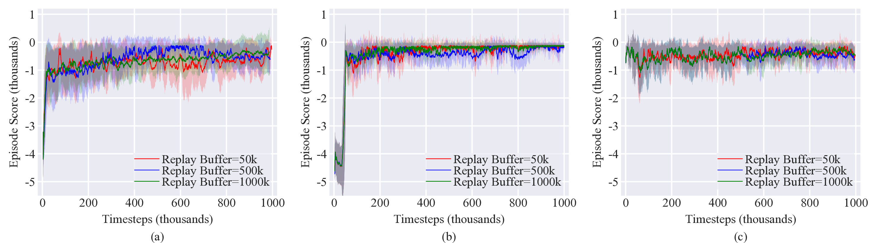
Limited hyperparameter tuning was performed for this case. The on-policy methods used the hyperparameters identified in Case 2 with a batch size of 16,000. For the off-policy methods, the replay buffer as well as the soft update coefficient $\tau$ were varied between two values. Results are shown in Figure 9. Hyperparameter tuning had little to no effect on the learning results as it was unable to enable the policy to explore the action space in such a way that the simulation was able to remain numerically stable.
RL methods for control of soft, compliant robots
For this work we selected five different deep RL algorithms. Specifically, we focused on model-free policy gradient methods. In the past few years, policy gradient methods with neural network function approximators have been shown to be successful for continuous control problems [1-3]. Also, compared with model-based RL approaches, model-free methods avoid the potential of exploiting bias in the learned model and are much easier to implement and tune.
Selected RL algorithms
The selected RL algorithms are Trust Region Policy Optimization (TRPO) [2], Proximal Policy Optimization (PPO) [3], Deep Deterministic Policy Gradient (DDPG) [1], Twin Delayed DDPG (TD3) [4] and Soft Actor-Critic (SAC) [5]. All selected algorithms are able to operate on a continuous action space, as is the case of our experiments.
Considering a standard RL framework setup, the learning agent interacts with an infinite-horizon discounted Markov Decision Process (MDP) defined by the tuple $(\mathcal{S}, \mathcal{A}, \mathcal{P}, r, \rho_0, \gamma)$, where the state space $\mathcal{S}$ and action space $\mathcal{A}$ are continuous. $\mathcal{P}$ denotes the state transition probability distribution, $r$ is the reward function, $\rho_0$ is the distribution of the initial state $s_0$, and $\gamma \in (0, 1)$ is the discounting factor.
In general, all selected algorithms optimize the expected cumulative discounted reward given initial state $s_0 \sim \rho_0$, discounting factor $\gamma$, policy $\pi$ and reward function $r : J(\theta, s_0) = E_{\pi \theta}\left[\sum_{t=0}^{\infty}\gamma^tr(s_t) \vert s_0\right]$ with respect to policy parameter $\theta$ using the policy gradient theorem [6].
Our selected implementations of TRPO and PPO perform policy updates while enforcing constraints to ensure stable training. The on-policy objective is formulated as $J(\theta) = E_t \left[ \frac{\pi_\theta(a_t \vert s_t)}{\pi_{\theta_{old}}(a_t \vert s_t)} \hat{A}_t \right]$, where $\hat{A}_t$ is an estimator of the generalized advantage function at timestep $t$ [2].
Specifically, TRPO uses the KL constraint $E_{t} \left[D_\text{KL}(\pi_{\theta_{old}}(.\vert s_t) | \pi_\theta(.\vert s_t)\right] \leq \delta$, while PPO uses a clipped surrogate objective function, which is similar to the TRPO constraint and comparatively easier to implement.
DDPG, TD3 and SAC are all off-policy actor-critic methods. They use sampled off-policy data to learn the Q-function and then use the Q-function to perform policy optimizations. While DDPG and TD3 learn the deterministic policy $\mu_\theta(s) = a$, SAC learns a stochastic policy $\pi_\theta(a \vert s) = Pr(a|s;\theta)$ based on entropy regularization. Additionally, TD3 is built upon DDPG and utilizes several tricks such as clipped double-Q learning (also used in SAC) to address the Q-value overestimation issue of DDPG.
Algorithm implementation and hyperparameter selection
To ensure proper implementation of the algorithms, we used the OpenAI stable-baseline implementations1. For each of the four cases considered, all algorithms were trained using 5 random seeds. The default parameters of the stable-baselines implementations are available online for TRPO2, PPO3, DDPG4, TD35, and SAC6. Unless noted, we used the default parameters from the stable-baseline implementations. Table 1 (TRPO), Table 2 (PPO), Table 3 (DDPG), Table 4 (TD3), and Table 5 (SAC) list the parameters that were changed from the default value. All training was performed using Stable Baselines v2.10.0 and Python v3.6.9.
| Parameter Description | Case1 | Case2 | Case3 | Case4 |
|---|---|---|---|---|
| Batch size | 1k–128k | 1k–128k | 16k | 16k |
| Parameter Description | Case1 | Case2 | Case3 | Case4 |
|---|---|---|---|---|
| Batch size | 1k–128k | 1k–128k | 16k | 16k |
| Parameter Description | Case1 | Case2 | Case3 | Case4 |
|---|---|---|---|---|
| Replay buffer size | 100k–2000k | 100k–2000k | 50k, 500k | 50k, 500k, 1000k |
| Soft update coefficient ( |
0.001 | 0.001 | 0.001, 0.005, 0.05 | 0.001 |
| Parameter Description | Case1 | Case2 | Case3 | Case4 |
|---|---|---|---|---|
| Replay buffer size | 100k–2000k | 100k–2000k | 50k, 500k | 50k, 500k, 1000k |
| Soft update coefficient ( |
0.005 | 0.005 | 0.001, 0.005, 0.05 | 0.005 |
| Learning starts | 50k | 50k | 50k | 50k |
| Parameter Description | Case1 | Case2 | Case3 | Case4 |
|---|---|---|---|---|
| Replay buffer size | 100k–2000k | 100k–2000k | 50k, 500k | 50k, 500k, 1000k |
| Soft update coefficient ( |
0.005 | 0.005 | 0.005, 0.05 | 0.005 |
Elastica implementation details
Details on Cosserat rod theory and the numerical discretization techniques used in Elastica are available in [7]; [8], however, here we will lay out some of the key implementation details for these problems such as how we set up and controlled the compliant arm, how contact is modeled in Elastica, and how Elastica treats internal friction and viscous dissipation.
Simulating and controlling a compliant arm with Elastica
The simulation of a soft, compliant robotic arm in Elastica consisted of a single Cosserat rod oriented vertically with a zero-displacement boundary condition applied to the element at the base of the rod to hold it in place. The physical parameters of the rod are given in Table 6. These parameters were held constant for all cases. Additional numerical parameters are given in Table 7. Consideration of the arm’s interaction with obstacles necessitated a more refined numerical discretization.
The simulation timestep required by Elastica is substantially smaller than what is necessary for the actor to control the arm. To address this, the timestep taken by Elastica and the update interval of the RL controller were decoupled with Elastica taking multiple timesteps between each update of the controller. The controller update interval was fixed at 1.4 ms for all cases.
To interface the Elastica simulation with the stable-baselines package, the Elastica simulation environment was developed to conform with the API format typical of OpenAI Gym problems7. This allows the cases presented here to be easily interfaced with any continuous control method that can work with Gym, hopefully spurring the development and benchmarking of new soft robot control algorithms. Beyond the flexibility to interface with a variety of control methods, the cases are capable of being run with different physical parameters, enabling further exploration of how the material and physical properties of a compliant robot influence its controllability.
| Parameter | Description | Value |
|---|---|---|
| Length of an undeformed arm [m] | ||
| Arm radius [cm] | ||
| Young’s modulus [MPa] | ||
| Dissipation coefficient [kg/(ms)] | ||
| Density [kg/ |
||
| Maximum torque [N.m] |
| Parameter | Description | Case 1 | Case 2 | Case 3 | Case4 |
|---|---|---|---|---|---|
| Number of discrete elements | |||||
| Elastica time-step [ms] | |||||
| RL time-step [ms] | |||||
| Episode duration (s) |
Arm actuation model
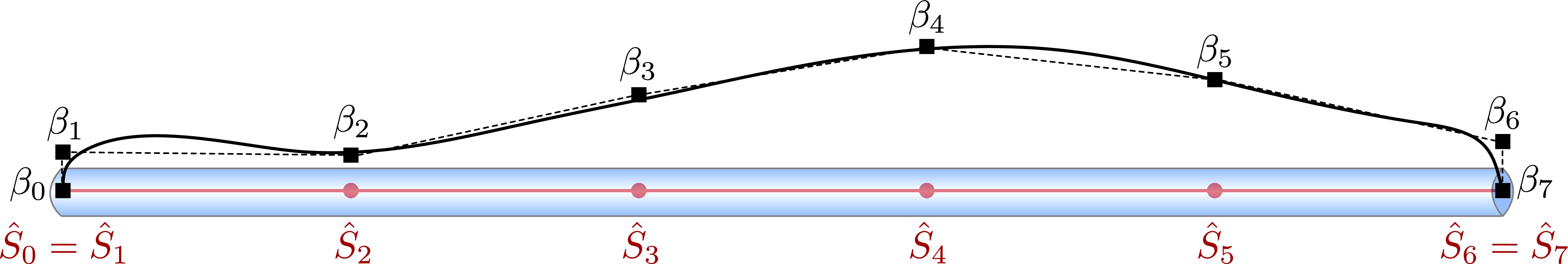
The actuation of the arm in all cases is achieved by application of orthogonal continuous torque profiles along the length of the arm. The torque profile $A_m(s)$ in the $m^{\text{th}}$-direction is expressed as $A_m({s})=\alpha_m \beta_m({s}),$ where $\alpha_m$ is the maximum torque, and $\beta_m({s})$ is the cubic spline passing through $N$ interpolation points $(\hat{S}_i,\beta_i)$ with $i=0,\dots,N-1$, as illustrated in Fig. 1. The first and last interpolation points are fixed so that $(\hat{S}_0,\beta_0)=(0,0)$ and $(\hat{S}_{N-1} , \beta_{N-1})=(\hat{L},0)$, therefore assuming the ends of the deforming body to be free.
The rest of the interpolation points $(\beta_{1},\dots,\beta_{N-2})$ are independently selected from a continuous action space bounded between $\left[-1,1\right]$ and scaled by $\alpha_m$ to get the applied torque curve. In the text, the term control points refers to the $(\beta_{1},\dots,\beta_{N-2})$ interpolation points selected by the controller.
These control points define the actions of the controller. An advantage of the proposed parameterization is that it encompasses a large variety of possible torque curves along the arm with a relatively small number of control points. Illustrating the convenience of the Cosserat mathematical formulation, it is possible to apply the actuation torques as external torques $\mathbf{c}={c_{1}, c_{2}, c_{3}}$, allowing a decoupling of passive and active stresses within the rod. Actuation torques are applied as ${c}_{m} = A_{m}$ where $m=1,2,3$ and represents the $\mathbf{d}_1$, $\mathbf{d}_2$, and $\mathbf{d}_3$ directions, respectively. The selected actuation torque is applied at each of the multiple Elastica timesteps that occur between RL controller updates.
Contact with solid boundaries
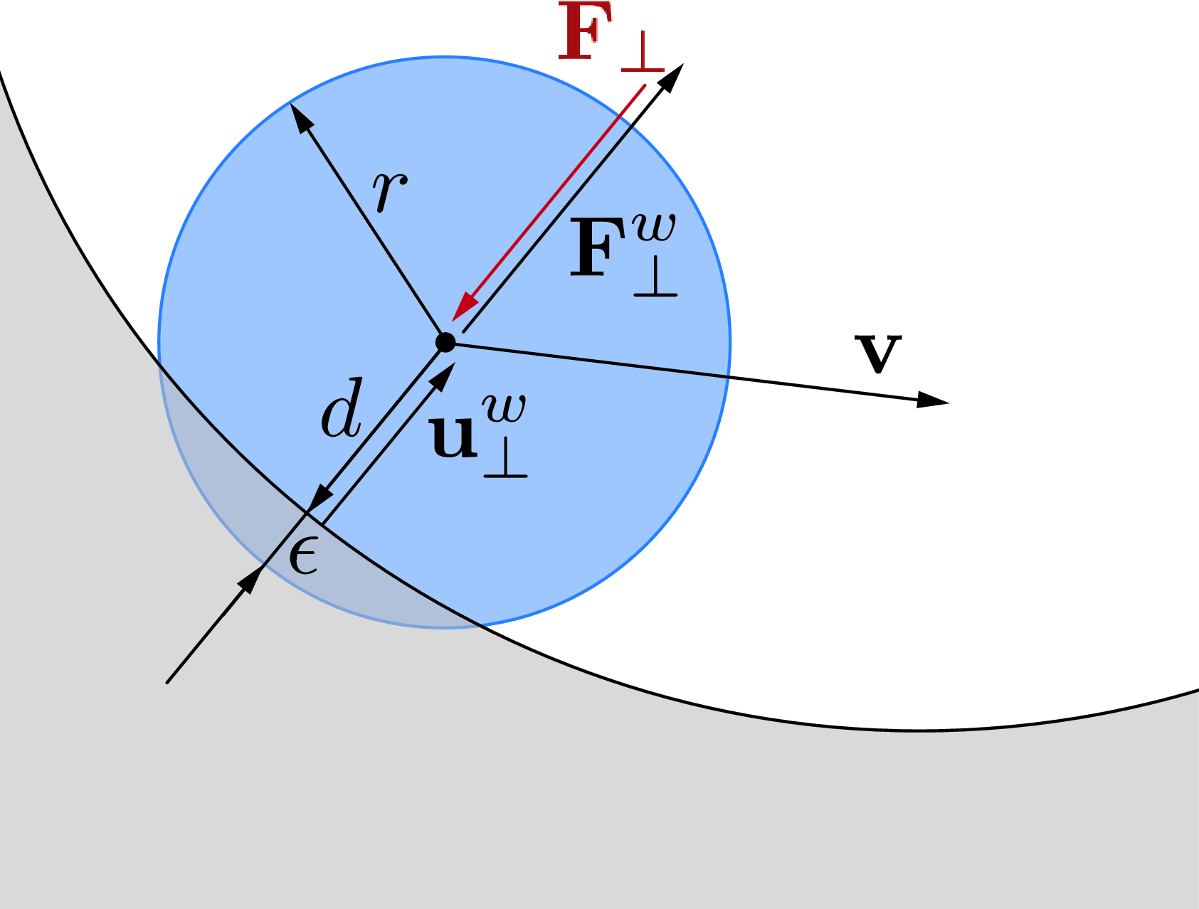
In order to investigate scenarios in which rods interact with the surrounding environment, we must also account for solid boundaries. Obstacles and surfaces are modeled as soft boundaries, allowing for interpenetration with the elements of the rod (Fig. 2). The wall response $\mathbf{F}^w_{\perp}$ balances the sum of all forces $\mathbf{F}_{\perp}$ that push the rod against the wall and is complemented by two other components which help prevent possible interpenetration due to numerics. The interpenetration distance $\epsilon$ triggers a normal elastic response proportional to the stiffness of the wall while a dissipative term related to the normal velocity component of the rod with respect to the substrate accounts for a damping force so that the overall wall response reads $\mathbf{F}^w_{\perp}= H(\epsilon)\cdot(-\mathbf{F}_{\perp} + k_w\epsilon-\gamma_w\mathbf{v}\cdot \mathbf{u}^w_{\perp})\mathbf{u}^w_{\perp}$ where $H(\epsilon)$ denotes the Heaviside function and ensures that a wall force is produced only in case of contact ($\epsilon\ge0$). Here $\mathbf{u}^w_{\perp}$ is the boundary outward normal (evaluated at the contact point, that is the contact location for which the normal passes through the center of mass of the element), and $k_w$ and $\gamma_w$ are, respectively, the wall stiffness and dissipation coefficients.
Dissipation
Real materials are subject to internal friction and viscoelastic losses, which can be modeled by modifying the constitutive relations so that the internal toques $\boldsymbol{\tau}(\boldsymbol{\kappa})$ and forces $\mathbf{n}(\boldsymbol{\sigma})$ become functions of both strain and rate of strain, i.e. $\boldsymbol{\tau}(\boldsymbol{\kappa}, \partial_t\boldsymbol{\kappa})$ and $\mathbf{n}(\boldsymbol{\sigma}, \partial_t \boldsymbol{\sigma})$. Keeping track of the strain rates increases computational costs and the memory footprint of the solver. However, for the purpose of purely dissipating energy, a simple alternative option is to employ Rayleigh potentials. In this case viscous forces $\mathbf{f}_v$ and torques $\mathbf{c}^v$ per unit length are directly computed as linear functions of linear and angular velocities through the constant translational $\gamma_t$ and rotational $\gamma_r$ internal friction coefficients, so that $\mathbf{f}_v=-\gamma_t\mathbf{v}$, and $\mathbf{c}^v=-\gamma_r\boldsymbol{\omega}.$ This approach does not model the physical nature of viscoelastic phenomena, although it does dissipate energy, effectively mimicking overall material friction effects. In the context of our numerical investigations, we did not observe any appreciable difference between the two outlined methods, so that, for the sake of simplicity and computational efficiency, we opted for the second one.
References
[1] Timothy P. Lillicrap, Jonathan J. Hunt, Alexander Pritzel, Nicolas Heess, Tom Erez, Yuval Tassa, David Silver, and Daan Wierstra. Continuous control with deep reinforcement learning, 2015.
[2] John Schulman, Sergey Levine, Philipp Moritz, Michael I. Jordan, and Pieter Abbeel. Trust region policy optimization. CoRR, abs/1502.05477, 2015.
[3] John Schulman, Filip Wolski, Prafulla Dhariwal, Alec Radford, and Oleg Klimov. Proximal policy optimization algorithms. CoRR, abs/1707.06347, 2017.
[4] Scott Fujimoto, Herke van Hoof, and David Meger. Addressing function approximation error in actor-critic methods. CoRR, abs/1802.09477, 2018.
[5] Tuomas Haarnoja, Aurick Zhou, Pieter Abbeel, and Sergey Levine. Soft actor-critic: Off-policy maximum entropy deep reinforcement learning with a stochastic actor. CoRR, abs/1801.01290, 2018.
[6] Richard S. Sutton, David Mcallester, Satinder Singh, and Yishay Mansour. Policy gradient methods for reinforcement learning with function approximation. In In Advances in Neural Information Processing Systems 12, pages 1057–1063. MIT Press, 2000.
[7] Mattia Gazzola, LH Dudte, AG McCormick, and L Mahadevan. Forward and inverse problems in the mechanics of soft filaments. Royal Society Open Science, 5(6):171628, 2018.
[8] Xiaotian Zhang, Fan Kiat Chan, Tejaswin Parthasarathy, and Mattia Gazzola. Modeling and simulation of complex dynamic musculoskeletal architectures. Nature Communications, 10(1):1– 12, 2019.
Footnotes
-
https://stable-baselines.readthedocs.io/en/master/modules/trpo.html ↩
-
https://stable-baselines.readthedocs.io/en/master/modules/ppo1.html ↩
-
https://stable-baselines.readthedocs.io/en/master/modules/ddpg.html ↩
-
https://stable-baselines.readthedocs.io/en/master/modules/td3.html ↩
-
https://stable-baselines.readthedocs.io/en/master/modules/sac.html ↩