Cosserat rods are a generalization of Kirchhoff rods, which model 1-d, slender rods incorporating only bend and twist. Cosserat rods add the ability to consider stretching and shearing, allowing all the possible modes of deformation of the system to be considered. The key assumption when modeling rods are that their length is much larger than their radius ($L \gg r$). This allows their dynamical behavior to be approximated by averaging balance laws at every cross-section. Other assumption are incompressibility and linearly elasticity (though non-linearities due to geometrical shape changes are captured).

Mathematical Description of Cosserat Rods

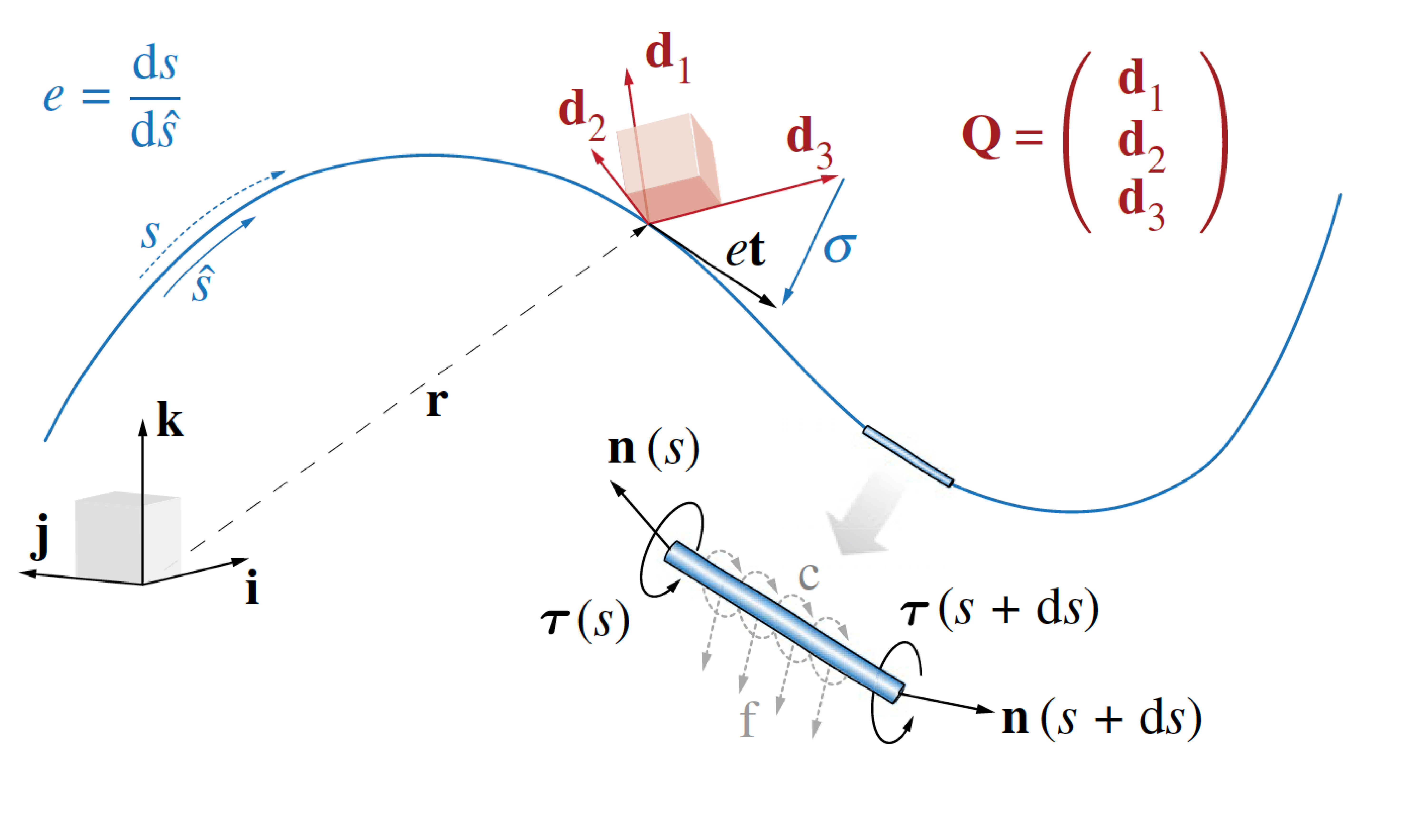
Cosserat rods are described by a centerline $\mathbf{r}(s, t)$ and local reference frame $\mathbf{Q}(s,t)= \{ {\mathbf{d}}_1, {\mathbf{d}}_2, {\mathbf{d}}_3 \}$, which consists of a triad of orthonormal basis vectors (using the right-hand rule convention). The dynamics of the rod are then described by the equations for conservation of linear and angular momentum throughout the rod.

Reference Frames

For a Cosserat rod described by a centerline $\mathbf{r}(s, t)$ (where $s \in [0, L]$ is the arc-length of the rod and $t$ is time) we begin by defining two reference frames within which we can express a vector $\mathbf{x}$:

The laboratory (Eulerian) frame: $\bar{\mathbf{x}} = x_1 \mathbf{i} + x_2 \mathbf{j} + x_3 \mathbf{k}$

The local (Lagrangian) frame: $\mathbf{x} = x_1 \mathbf{d}_1 + x_2 \mathbf{d}_2 + x_3 \mathbf{d}_3$

We can define a rotation matrix $\mathbf{Q}$ between these two reference frames as $\mathbf{Q}= \{ {\mathbf{d}}_1, {\mathbf{d}}_2, {\mathbf{d}}_3 \}$, allowing us to convert between the laboratory and local reference frames via $\mathbf{x}=\mathbf{Q}\bar{\mathbf{x}}$ and $\bar{\mathbf{x}}=\mathbf{Q}^T \mathbf{x}$. The local frame describes the orientation of the rod where ${\mathbf{d}}_3$ points along the centerline tangent ($\partial_s \bar{\mathbf{r}}=\bar{\mathbf{r}}_s= e \bar{\mathbf{t}}$) when there is no shear while ${\mathbf{d}}_1$ and ${\mathbf{d}}_2$ span the normal-binormal plane.

If there is shear or extension, then ${\mathbf{d}}_3$ is shifted away from the tangent vector by some amount. This can be described by a shear strain vector $\boldsymbol{\sigma}= \mathbf{Q}\bar{\mathbf{r}}_s - \mathbf{d}_3$ in the local frame. Additionally, when there is shear or extension, it is important to distinguish between the reference configuration ($\hat{s}$) and the deformed configuration ($s$). The stretch ratio between the two states is defined as $e=\frac{\mathrm{d} s}{\mathrm{d}\hat{s}}$. If we define a unit tangent vector $\bar{\mathbf{t}}$, we can now represent the local orientation of the rod as $\bar{\mathbf{r}}_s= e \bar{\mathbf{t}}$. Along with shear strain, the rod can also twist and rotate. In the local (Lagrangian) reference frame, as we move along the rod, our reference frame $\mathbf{Q}(s,t)$ is continually changing. This change represents the curvature of the rod and is represented with a curvature vector $\boldsymbol{\kappa}$, which is defined as $\partial_s \mathbf{d}_j = \boldsymbol{\kappa} \times \mathbf{d}_j$.

Now that we have established our reference frames, the next thing we need to do is define how we are going to track changes in the shape of the rod. The change in $\mathbf{Q}(s,t)$ over time defines the angular velocity $\boldsymbol{\omega}$ of the rod ($\partial_t \mathbf{d}_j = \boldsymbol{\omega} \times \mathbf{d}_j$). We also want to define the translational velocity at each point of the centerline of the rod. We do this by defining velocity as $\bar{\mathbf{v}} = \partial_t\bar{\mathbf{r}}$.

Finally, there are a number of material and structural parameters that need to defined such as the mass per unit length ($\rho$). These parameters are defined in the reference ($\hat{s}$) configuration and scaled by the stretch ratio $e$. They are:

• cross-sectional area: $A = \frac{\hat{A}}{e}$
• bending stiffness matrix: $\mathbf{B} = \frac{\hat{\mathbf{B}}}{e^2}$
• shearing stiffness matrix: $\mathbf{S} = \frac{\hat{\mathbf{S}}}{e}$
• second area moment of inertia: $\mathbf{I} = \frac{\hat{\mathbf{I}}}{e^2}$

Conservation of Momentum

With all these terms defined, we can now define the balance laws that need to be satisfied at every cross-section. By balancing both linear and angular momentum at every cross-section we are able to describe the dynamics of the Cosserat rod. For a prescribed external force and couple line density ($\bar{\mathbf{f}}$ and $\mathbf{c}$, respectively) the momentum balance equations are:

Linear Momentum: $\small{\rho A \cdot \partial_t^2 \bar{\mathbf{r}} = \overbrace{\partial_s \left( \frac{\mathbf{Q}^T \mathbf{S} \boldsymbol{\sigma}}{e} \right)}^{\substack{\text{internal shear/} \\ \text{stretch force}}} + \overbrace{e \ \bar{\mathbf{f}}}^{\substack{\text{external} \\ \text{force}}} }$

Angular Momentum: $\small{\begin{align} \frac{\rho \mathbf{I}}{e} \cdot \partial_t \boldsymbol{\omega} =&\overbrace{\partial_s \left( \frac{\mathbf{B} \boldsymbol{\kappa}}{e^3} \right) + \frac{\boldsymbol{\kappa} \times \mathbf{B} \boldsymbol{\kappa}}{e^3}}^{\text{internal bend/twist couple}} +\overbrace{\left( \mathbf{Q}\frac{\bar{\mathbf{r}}_s}{e} \times \mathbf{S} \boldsymbol{\sigma} \right)}^{\substack{\text{internal shear/} \\ \text{stretch couple}}} + \\&\underbrace{\left( \rho \mathbf{I} \cdot \frac{\boldsymbol{\omega}}{e} \right) \times \boldsymbol{\omega}}_{\text{Lagrangian transport}}^{\phantom{o}} +\underbrace{\frac{\rho \mathbf{I} \boldsymbol{\omega}}{e^2} \cdot \partial_t e}_\textrm{unsteady dilation} + \underbrace{e \ \mathbf{c}}_{\substack{\text{external} \\ \text{couple}}} \end{align}}$

Solving these equations, along with appropriate boundary conditions, allows us to model the dynamics of a single Cosserat rod. In general, there is not always an analytical solution to these equations. Instead, we use numerical methods to solve for these dynamics. For information on the numerical method we use, see here. If we want to examine how multiple rods interact, we also need to define the interactions and connections between these rods. More information on how to connect multiple rods to form an assembly of rods may be found here.

A note on notation: We have created a pdf with a list of the different variables we use and their definitions available for download here.

Linear Elasticity

To solve the momentum balance equations, we needed to define a bending stiffness ($\mathbf{B}$) and shearing stiffness ($\mathbf{S}$). We are assuming that the rod is a perfectly elastic material with a linear stress-strain response. For an elastic beam, these stiffness matrices are diagonal 3x3 matrices:

$\mathbf{B} = \begin{bmatrix} E \ I_1 & & \\ & E \ I_2 & \\ & & G \ I_3 \end{bmatrix} \quad \text{ and } \quad \mathbf{S} = \begin{bmatrix} \alpha_c G \ A & & \\ & \alpha_c G \ A & \\ & & E \ A \end{bmatrix}$

Here $E$ is the elastic Young’s modulus, $G$ is the shear modulus, $I_i$ is the second area moment of inertia, $A$ is the cross sectional area and the constant $\alpha_c$ is $4/3$ (for circular cross sections). Additionally, because of the linear elastic assumption, we can define constitutive laws for both the load-strain relations as well as the torque-curvature relations. These are:

Load-strain: $\mathbf{n} = \mathbf{S}(\boldsymbol{\sigma} - \boldsymbol{\sigma^0})$

Torque-curvature: $\boldsymbol{\tau} = \mathbf{B}(\boldsymbol{\kappa} - \boldsymbol{\kappa^0})$

$\boldsymbol{\sigma^0}$ and $\boldsymbol{\kappa^0}$ are reference curvatures that allow the rod to have a stress-free configuration in shapes other than a straight line.

Useful References

Gazzola, Dudte, McCormick, Mahadevan, Forward and inverse problems in the mechanics of soft filaments, Royal Society Open Science, 2018.

Zhang, Chan, Parthasarathy, Gazzola, Modeling and simulation of complex dynamic musculoskeletal architectures, Nature Communications, 2019.